So I’ve got this web-based image gallery. The images in it are organized with simple tags (there’s a many-to-many relationship between images and tags). Every image has at least one tag, and almost all images have several tags. When a user wants to look up an image in the gallery, they select one or more tags and are shown thumbnails for all images which have at least those tags. At first the image thumbnails were simply sorted alphabetically by file name, and this worked fine when the size of the collection was modest, but that didn’t last. Soon the collection grew to the point where most queries would give forty or more thumbnails, and it became pretty challenging to find your desired image in the pile. The search was even trickier if you had only a general idea of what you were looking for and couldn’t select lots of tags to narrow things down.
To improve the usability of this thing I had to come up with a way to arrange the image thumbnails in a particular order such that images with similar characteristics were placed near each other. This would make it much, much easier to visually scan the mass of thumbnails. In this post I’ll elaborate on the technical details of the problem and how I developed the algorithm I’m currently using.
First thing’s first, how do you quantify the similarity of two images? Well, images with exactly the same tags should obviously be adjacent, so the problem can be changed a little to reduce the number of items that need to be arranged: identically-tagged images can be gathered into groups, and then these groups can be arranged by similarity. Each group is defined by the tags that belong to the image or images in it, a distinct subset of all tags in the system.
Groups with tags in common should be near each other, naturally, so the cardinality of the set intersection is definitely a candidate for our similarity metric. The number of tags in a group’s set varies significantly in this application (some images may have half a dozen or more tags while others may have only one), so in order to compare values properly our metric should probably be normalized in some way. This line of reasoning leads to the Jaccard index:
![]()
Identical sets have J=1, disjoint sets have J=0, and all other cases fall somewhere in between. Closely related is the Jaccard distance:
![]() … which is trivially harder to calculate and makes the space of tag subsets a metric space, which has several nice properties. In particular, the Jaccard distance satisfies the triangle inequality, which could come in handy when trying to generate a solution to this problem efficiently. We’re now talking about minimizing distance rather than maximizing similarity, but that’s just semantics. There are no infinite distances; if necessary any two groups can be neighbors. Speaking of which, will it always be possible to arrange the groups in such a way that every tag appears in a contiguous block? No sir. It only takes three groups and three tags to construct a case where total continuity is impossible.
… which is trivially harder to calculate and makes the space of tag subsets a metric space, which has several nice properties. In particular, the Jaccard distance satisfies the triangle inequality, which could come in handy when trying to generate a solution to this problem efficiently. We’re now talking about minimizing distance rather than maximizing similarity, but that’s just semantics. There are no infinite distances; if necessary any two groups can be neighbors. Speaking of which, will it always be possible to arrange the groups in such a way that every tag appears in a contiguous block? No sir. It only takes three groups and three tags to construct a case where total continuity is impossible.
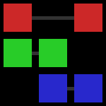 In this grid-style visualization, the columns are sets of tags, or groups, and each distinct tag is marked in its own row and has its own color. Just to be clear, the first group has tags red and green, the second has tags green and blue, and the third has tags red and blue. Gray lines show the range over which each tag spans, obviating the red tag’s gap. You can see that no matter how you arrange these three groups there will always be one tag with a discontinuity. So it’s futile to try to develop an algorithm which achieves total continuity, which is good to know.
Putting the problem in terms of graph theory, what we have is a complete graph where the vertexes are groups of identically-tagged images and the edges are weighted with the Jaccard distances between the sets of tags for the groups they connect. What we want is a Hamiltonian path in this graph having minimum cost. The similarity of this problem to the old classic the traveling salesman problem is evident. The only difference between this problem and TSP is that a solution for TSP is a Hamiltonian cycle rather than a path. Knowing that we’re dealing with a metric space means we can apply existing TSP heuristics which depend on that constraint. So, can we simply solve for TSP and then drop the most expensive edge from the cycle to get an optimal path? Nope.
 In this example case the optimal Hamiltonian path is A-B-C-D with total cost 3. An optimal Hamiltonian cycle is A-B-D-C-A with total cost 6, and dropping one of the most expensive edges to reduce this to an open path gives e.g. A-B-D-C with total cost 4. Now, the costs of these edges don’t satisfy the triangle inequality as the Jaccard distance does, but even if the edge with weight 100 instead had weight 3 the aforementioned cycle would still be optimal, so finding an optimal cycle and then omitting the most expensive edge is not guaranteed to yield an optimal open path. So TSP isn’t the best place to start. (update: I have actually figured out a much better way to map the problem. More in a future post.)
The first algorithm I came up with I’ll call the insert algorithm. The general idea is to construct the sequence of groups by inserting groups into it one at a time wherever they fit best at the time. The procedure looks like this:
|
1 2 3 4 5 6 7 8 9 10 11 12 13 14 15 16 17 18 19 20 |
f_cost = lambda (l, g, r):\ 0 if not g or (not l and not r) else\ f_jaccdist((l,g)) + f_jaccdist((g,r)) if l and r else\ f_jaccdist((l,g)) * 2 if l else\ f_jaccdist((g,r)) * 2 orderedgroups = [] groups = sorted(groups, key=len, reverse=True) while groups: best = None # (group, position, cost) for g in groups: for p in xrange(0, len(orderedgroups) + 1): cost = f_cost(( orderedgroups[p-1] if p > 0 else None, g, orderedgroups[p] if p < len(orderedgroups) else None)) if best == None or cost < best[2]: best = (g, p, cost) orderedgroups.insert(best[1], best[0]) groups.remove(best[0]) |
This thing comes up with an ordering that’s pretty OK, certainly much better than random. What about time complexity, though? Well with three nested loops it shouldn’t be surprising that the complexity is tightly bound by a function of N^3 where N is the number of groups. That could be worse, but remember this is for a web application, and my web server happens to be an Atom D525. The application’s image collection never stops growing, and this algorithm wouldn’t stay feasible for long.
I tried to speed things up with some simple memoization. Notice that on the order of N^3 Jaccard distances are evaluated, but there are only N-choose-2 (less than N^2) distinct distances among all the groups. I modified the above code to calculate all distances a-priori and store them in a dictionary. As it turns out those calculations aren’t all that expensive in Python, so the gain was pretty marginal:
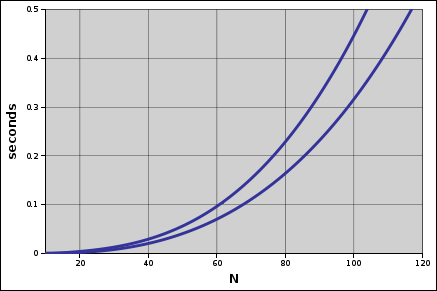 Taking 200 milliseconds as the longest acceptable run time, memoization stepped up the maximum feasible number of groups from about 75 to 85 for this algorithm. Calculating the distances up front didn’t secure this algorithm’s place in the future, but it did lead me into a new line of thought.
If the distances are all going to be calculated anyway, how about, instead of using those values to decide where to place each group, we use those values to choose which pairs of groups are adjacent? In other words, going back to the graph model, choose edges from the graph least-cost-first until all vertexes are connected. In terms of sequences of groups, the idea is to start with N sequences of length 1 (each group in its own sequence) and then connect these sequences end-to-end until there is one sequence of length N. I call this the assembler algorithm. There’s too much code to illustrate with short snippets, so here is the complete implementation: imgez-ordering.py
The meat of this thing is a heap, with heaps nested and indexed-into in various ways in order to accelerate the particular discard operations needed to assemble the sequences. Being little more than a sort of N-choose-2 items, this algorithm runs in time N^2*log(N) and is dramatically faster than the insert algorithm:
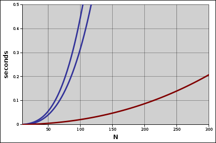 With the same 200 millisecond cutoff, the assembler is useful for up to 300 groups, a 250% improvement. Speed is nice, but quality is nicer. Let’s see how these two algorithms compare with some real data.
The following visualizations are done in the same style as the 3-by-3 example above. Each column in the grid is a group, each tag has its own color and row, and gray lines connect the most distant instances of each tag.
First, the groups in random order:
Next, the same groups run through the insert algorithm:
And finally, the assembler algorithm:
The assembler wins. It’s fast, and it’s good.


